Multiples, most notably the EV/EBITDA multiple, are universally used in private equity to value companies. In contrast, the theoretical correct valuation approach, the discounted cash flow model (DCF), is rarely found in LBO models, pitch books, etc. Of course, there are good reasons for this, nicely summarized by Liu/Nissim/Thomas (2002):
While the multiple approach bypasses explicit projections and present value calculations, it relies on the same principles underlying the more comprehensive approach: value is an increasing function of future payoffs and a decreasing function of risk. Therefore, multiples are used often as a substitute for comprehensive valuations, because they communicate efficiently the essence of those valuations. Multiples are also used to complement comprehensive valuations, typically to calibrate those valuations to obtain terminal values.
Put differently, multiples can be thought of as a summary statistic of a comprehensive valuation that is helpful in communicating the essence. A summary statistic typically does not contain the same amount of information as the data that is summarized, and one therefore has to be careful with regards to how and when to use it. Otherwise, one can end up such as the statistician who drowned in a lake averaging only 2 inches in depth…
In this post, I derive under certain simplifying assumptions the EV/EBITDA multiple from a DCF model and discuss the factors that drive the EV/EBITDA multiple. I then discuss the consequences if those simplifying assumptions do not hold. In the blog post “EV/EBITDA valuation multiple: the data”, I look at the issue empirically.
Starting with a DCF of all expected free cash flows \(FCFF\), the enterprise value at time \(t\), \(EV_t\), can be written as:
\[ EV_t = \sum_{i=t+1}^{\infty} \frac{FCFF_i}{(1+r)^i}, \] where \(r\) is the firm-specific discount rate. For simplicity, I ignore the expectation operator \(E()\).
\(FCFF_i\) can be rewritten as follows:1
\[ FCFF_i = (EBITDA_i - DA_i) \times (1 - \tau) + DA_i - \Delta NWC_i - CAPEX_i, \\ \]
where \(DA\) is depreciation & amortization, \(CAPEX\) is capital expenditure and \(\tau\) is the tax-rate. \(\Delta NWC\) is the change of the net working capital in the period. If \(NWC\) increases, it will reduce \(FCFF\).
This formula shows nicely why EBITDA is so prominent in private equity in the first place: it is a proxy for cash flows that is less impacted by periodic items such as D&A and net working capital changes. However, one must remember that EBITDA ignores capital expenditures. As Warren Buffett apparently once asked: “Does management think the tooth fairy pays for capital expenditures?”
Let’s come to this point later, but let’s first make some simplifying assumptions:
- Depreciation & amortization, \(DA\), equals capital expenditures, \(CAPEX\)
- The change in net working capital, \(\Delta NWC\), is 0
As the difference between D&A and capital expenditures as well as changes in net working capital are transitory, these assumptions should hold in the long run. We can then rewrite the above equation:
\[ \begin{aligned} FCFF_i &= (EBITDA_i - DA_i) \times (1 - \tau) \\ &= EBITDA_i \times (1-\frac{DA_i}{EBITDA_i}) \times (1-\tau) \\ &= EBITDA_i \times OCC_i \times (1-\tau), \end{aligned} \]
where \(OCC_i\) is the operational cash conversion. If it is close to 100%, it means that most EBITDA ends up in the firm’s debt- and equity holders’ pockets. If it is close to 0% due to high capital requirements, a lot of cash must be invested to generate the EBITDA.
Let’s add two more assumptions:
- Operational cash conversion stays constant over time, i.e. \(OCC_i=OCC_{i+1}=...=OCC\)
- EBITDA grows by a constant factor \(g\)
We can now rewrite the calculation of \(EV_t\):
\[ \begin{aligned} EV_t &= \sum_{i=t+1}^{\infty} \frac{EBITDA_i \times OCC_i \times (1-\tau)}{(1+r)^i} \\ &= \sum_{i=t+1}^{\infty} \frac{EBITDA_t \times OCC \times (1-\tau)\times (1+g)^i}{(1+r)^i} \\ &= \frac{EBITDA_t \times OCC \times (1-\tau) \times (1+g)}{r-g}, \end{aligned} \]
or
\[ \frac{EV_t}{EBITDA_t} = \frac{OCC \times (1-\tau) \times (1+g)}{r-g} \]
In words, the EV/EBITDA multiple is a function of the operational cash conversion \(OCC\), the growth of the business, \(g\), 1 minus the tax rate, and the discount rate, \(r\). All else being equal, the multiple is the higher,
- the more cash generative the business;
- the higher the growth of the business;
- the lower the tax rate; and
- the lower the discount rate, i.e., the risk of the business.
Ignoring taxes by setting \(\tau=0\), I plot the EV/EBITDA multiple in relation to the other three factors below.
Show code
library(data.table)
library(ggplot2)
DT <- as.data.table(expand.grid(OCC = seq(from=0.0,  to=1,   by=0.1),
                                g   = seq(from=0.0, to=.05, by=0.001),
                                r   = seq(from=0.1,  to=.15, by=0.01)))
DT[, Multiple:=OCC*(1+g)/(r-g)]

DT[, OCC:=as.factor(OCC)]
DT[, r  :=as.factor(r)]

ggplot(DT, aes(x=g, y=Multiple, color=OCC)) +
  geom_line() +
  facet_wrap(~r) +
  scale_x_continuous(labels = scales::percent) +
  xlab("Steady-state growth rate") + ylab("EV/EBITDA multiple") +
  labs(title="EV/EBITDA multiple as function of operational cash conversion (OCC),\n steady-state growth and discount rate",
       caption = "The values in the group boxes indicate the discount rate")
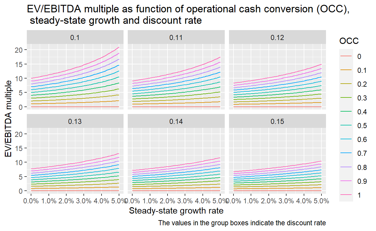
Starting with the operational cash conversion, note that the EV/EBITDA multiple is 0x in case of a 0%-cash conversion. This is not surprising: if a business does not generate any cash on top of what it must re-invest in capital, it should be worth zero. More generally, businesses in sectors with high cash generation (e.g., software) should have much higher valuation multiples as businesses in CAPEX-intensive sectors such as manufacturing. The growth rate is also an important factor. Going from a 0% p.a. growth rate to a 5% p.a. roughly doubles the EV/EBITDA multiple in case of lower discount rates. Finally, the higher the discount rate, which can for example be calculated with the Weighted-Average Cost of Capital (WACC) method, the lower the valuations. A change from 10% to 15% might not sound like much, but it lowers an EV/EBITDA of a business with 100% OCC and 5% p.a. growth from over 20x to just around 10x (see right end of the most upper curve in the top left vs. the bottom right chart).
These relationships are very important to keep in mind when valuing a business with the multiple approach. For example, if you are looking at a company that has a much lower cash-generation than its peers, it should have a much lower valuation. Applying the same EV/EBITDA multiple as the peers can lead to large valuation mistakes.
Furthermore, remember that we needed quite a bit of simplifying assumptions to establish the relationship between the FCFF-DCF method and the EV/EBITDA multiple. These assumptions most certainly will not hold for an actual business. For example, it is not easy to translate future growth over many periods in one reasonable assumption for \(g\).
The attentive reader will notice that the tax is calculated based on the EBIT, the earnings before interest, which is incorrect, as it is in reality based on the EBT, the earnings after interest. In the DCF model, the tax benefits of debt and the accompanying interest are considered in the discount rate, which makes the calculation much simpler. Hence, \(\tau\) has to be considered as a hypothetical tax rate, not the actual one, yet another simplification.↩︎