Modelling cash flows of private equity funds is important for investors, especially for liquidity management. Unfortunately, it is also difficult. An important question an investor has to ask is what model to use. In the end, all models are simplifications of reality, but there is a huge variety on what assumptions are made, which parameters are important, and which are ignored.
In this post, I’m presenting one of the earliest models for fund cash flows, the Takahashi and Alexander (TA) model, and show how to implement it in R. Introduced in Takahashi and Alexander (2002) over two decades ago, it is still used in the industry today. This success stems in my opinion from its simplicity: the model can be described with a few simple equations and easily be implemented in tools such as Excel and R in a few minutes to draw nice-looking curves of capital calls and distributions.
This simplicity makes the model quite useful for quick analyses. Sometimes, all you need is a capital call and distribution curve of a fund to test out a few hypotheses such as what the gross/net spread of a fund should be with certain fee and carry terms. In the next section, I outline the relevant equations. I thereby follow the notation of Jeet (2020), who provides a nice introduction as well as a helpful modification to the model.
The Takahashi and Alexander model
There are three vectors an investor is interested about a PE fund: a vector of capital calls, distributions, and NAVs. The TA model starts by defining the capital call in period \(t\), \(C_t\), as the uncalled commitment at the end of the previous period, \(UC_{t-1}\), multiplied with a rate of contribution, \(RC\), that is a function of the age of the fund:
\[ C_t = UC_{t-1} \times RC(Age_{t-1}). \]
TA give some guidance on how to specify RC: “Rather than specify a different rate of contribution every year, we simplify the model by separating the first two years of contributions from subsequent years. Typically, we would assume two similarly sized large contributions in years one and two, and geometrically declining contributions in subsequent years.” Of course, one can deviate from this. For example, I don’t see a good reason to separate between the first two years and subsequent years and would rather separate between the investment period (typically 3-5 years) and thereafter.
Distributions in \(D_t\) are the product of the NAV at the end of the previous period, \(NAV_{t-1}\), multiplied with a growth rate, \(G_t\),1 and a rate of distribution function \(RD\):
\[ D_t=NAV_{t-1} \times (1+G_t) \times RD(Age_t-1, bow, L). \] In contrast to the RC function, TA specify the RD function, which is the defining characteristic of their model. Concretely,
\[ RD=\left(\frac{Age_{t-1}}{L} \right)^{bow}. \]
Below I plot the RD function for different \(bow\) values to get a better understanding of the mechanics. A few observations:
- The rate of distribution increases over time and always ends up at 100%
- The higher the \(bow\) factor, the lower the rate of distribution is in earlier years
- A \(bow\) factor of 1 is the special case for which the rate of distribution increases linearly with the age of the PE fund
Show code
library(data.table)
library(ggplot2)
RD_function <- function(age, L, bow) {
  return((age/L)^bow)
}
vecBow <- seq(from=0.5,to=3,by=0.5)
vecAge <- 1:15
rdDT <- data.table(Bow = rep(vecBow, each=length(vecAge)),
                   Age = rep(vecAge, times=length(vecBow)))
rdDT[, RD:=RD_function(age=Age, bow=Bow,L=max(Age)), by=Bow]

ggplot(rdDT, aes(x=Age, y=RD)) +
  geom_line() +
  facet_wrap(vars(Bow), nrow=3) +
  ylab("Rate of Distribution (RD)")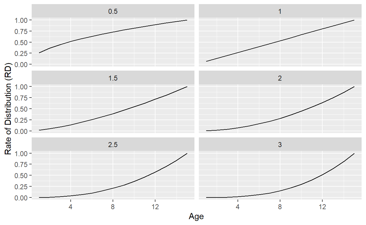
Figure 1: Rate of distribution (RD) in the TA model for different bow factors.
Implementation in R
Below is the code for an R function to run the TA model in R, together with a function that produces outputs, including ggplot2 plots:
Show code
# This file includes functions to run the Takahashi / Alexander (TA) model

#' This function produces vectors of contributions, distributions, and NAVs,
#' based on the deterministic Takahashi / Alexander (TA) (2002) model and
#' adjusted for a periodically changing growth rate, as proposed by
#' Jeet (2020).
#'
#' The inputs of the model are explained in the parameter section. The
#' inputs have to be adjusted based on the desired periodicity (annually,
#' quarterly, etc.).. Three equations fully describe the model:
#'
#' Equation to model capital calls \eqn{C_t} in period t, based on
#' uncalled capital \eqn{UC_t}:
#'
#' \deqn{C[t] = UC[t] * .vec\_RC[t]}
#'
#' \code{.vec_RC} is the vector of rate of contributions. This one is pretty
#' straightforward; the called capital in a period is the beginning-of-period
#' uncalled capital multiplied with the percentage of capital assumed /
#' expected to be called in the period.
#'
#' To model distributions \eqn{D_t} in period t, the following equation is
#' used:
#'
#' \deqn{D[t] = NAV[t-1] * (1+.vec\_growth[t]) * RD(Age[t-1],.bow,.life)}
#'
#' The distributions have to come from the NAV of the fund, which is grown
#' by a growth factor over time. The level of distributions is then defined
#' by a function RD as follows:
#'
#' \deqn{RD = (\frac{Age[t-1]}{.life})^{.bow}}
#'
#' The term in brackets linearly increases from 0 to 1 over the fund's
#' life time \code{.life}. With the \code{.bow} factor, the modeler can
#' control how front or backloaded those distributions are. The higher
#' the bow factor, the smaller RD becomes as the factor in brackets is
#' typically below 1.
#'
#' The NAV is modeled simply by growing it with the growth factor and
#' adjusting for distributions and capital calls:
#'
#' \deqn{NAV[t] = NAV[t-1]*(1+vec_growth[t]) + C[t] - D[t]}
#'
#'
#' @param .bow numeric; defines the distribution rate over the life of the
#'        investment. A higher bow factor projects more distributions
#'        occurring later in the investment’s life.
#' @param .life numeric; the term / lifetime of the fund.
#' @param .vec_growth numeric vector; growth vector of the NAV; user can
#'        also only supply a scaler / one number, in which case a constant
#'        growth rate is assumed.
#' @param .vec_RC numeric vector; vector of rate of contributions. Valid inputs
#'         are between 0 and 1.
#' @param .nav numeric; NAV at the beginning; default value is 0, which implies
#'         that the full term of the fund is modeled; however, the TA model
#'         can also be applied to funds that are already older than age 0.
#' @param .uc numeric; uncalled capital; for a new fund (e.g.\code{.nav=0}),
#'        this value is equal to the commitment amount.
#' @return A data.table holding all the relevant information of the fund:
#'         Inputs of TA model: Age, bow factor, rate of contributions, growth rate
#'         Outputs of TA model: calls and distributions (also cumulated); NAV
#'         and uncalled capital both at the beginning of the period (BOP) and
#'         end of period (EOP).
#'
#' @export
#'
#' @references
#' Takahashi / Alexander (2002): Illiquid Alternative Asset Fund Modeling,
#' The Journal of Portfolio Management
#' Jeet (2020): Modeling Private Investment Cash Flows with
#' Market-Sensitive Periodic Growth, PGIM
#'
#' @examples
#' # Taken from Jeet (2020): Modeling Private Investment Cash Flows
#' # with Market_Sensitive Periodic Growth
#' run_TA_model(.bow=2,
#'              .life=13,
#'              .nav=0,
#'              .uc=1,
#'              .vec_growth = c(0.05,0.04,0.06,0.01,-0.01,0.02,
#'                              0.07,0.08,0.02,0.05,0.07,0.02,0.03),
#'              .vec_RC = c(0.25,0.33,rep(0.5,11)))
#' # Run it quarterly (not quite the same as above, as cash flows are not
#' # compouned for a full year anymore)
#' run_TA_model(.bow=2,
#'              .life=13*4,
#'              .nav=0,
#'              .uc=1,
#'              .vec_growth = rep(c(0.05,0.04,0.06,0.01,-0.01,0.02,
#'                              0.07,0.08,0.02,0.05,0.07,0.02,0.03),
#'                              each=4)/4,
#'              .vec_RC = rep(c(0.25,0.33,rep(0.5,11)),
#'                        each=4)/5)
#' # Model fund that is already running for a few years
#' run_TA_model(.bow=2,
#'              .life=7,
#'              .nav=0.8,
#'              .uc=0.15,
#'              .vec_growth = rep(0.07, times=7),
#'              .vec_RC =     rep(0.75,times=7))
run_TA_model <- function(.bow, .life, .vec_growth, .vec_RC,
                         .nav = 0, .uc) {


  ####### Checks
  #'#################################################################################
  # Check that .vec_growth and .vec_RC are the same length
  len <- length(.vec_growth)
  #If user used scalar, create vector with same length as .vec_RC
  if (len==1) {
    .vec_growth <- rep(.vec_growth, times=length(.vec_RC))
  } else if (len!=length(.vec_RC)) {
    stop("run_TA_model: .vec_growth and .vec_RC not of same length.")
  } else if (length(.vec_RC)!=.life) {
    stop("run_TA_model: the length of .vec_RC has to be the same as .life")
  }

  #'#################################################################################
  # Check that assumptions are reasonable
  if (!is.numeric(.bow) | .bow<0 | length(.bow)!=1) {
    stop("Bow factor .bow should be numeric, not a vector, and non-negative.")
  }
  if (!is.numeric(.life) | .life<0 | length(.life)!=1 | .life<2) {
    stop("Life .life should be numeric, not a vector, larger than 1, and non-negative.")
  }
  if (!is.numeric(.nav) | .nav<0 | length(.nav)!=1) {
    stop("NAV .nav should be numeric, not a vector, and non-negative.")
  }
  if (!is.numeric(.uc) | .uc<0 | length(.uc)!=1) {
    stop("Uncalled capital .uc should be numeric, not a vector, and non-negative.")
  }

  ### Calculate the vector of rate of distributions
  vec_RD <- ((1:.life)/.life)^.bow

  ### Initialize vectors
  vec_CC  <- numeric(.life)
  vec_D   <- numeric(.life)
  vec_NAV <- numeric(.life+1)
  vec_UC  <- numeric(.life+1)
  vec_NAV[1] <- .nav
  vec_UC[1]  <- .uc

  ### Loop through each period to calculate values
  for (t in 1:.life) {
    vec_CC[t] <- vec_UC[t] * .vec_RC[t]
    vec_D[t]  <- vec_NAV[t] * (1+.vec_growth[t])*vec_RD[t]
    vec_NAV[t+1] <- vec_NAV[t] * (1+.vec_growth[t]) + vec_CC[t] - vec_D[t]
    vec_UC[t+1]  <- vec_UC[t] - vec_CC[t]
  }

  return(data.table::data.table(Age      = 1:.life,
                                Bow      = .bow,
                                RC       = .vec_RC,
                                Growth   = .vec_growth,
                                Calls    = vec_CC,
                                Dist     = vec_D,
                                CumCalls = cumsum(vec_CC),
                                CumDist  = cumsum(vec_D),
                                NAV_BOP  = vec_NAV[1:.life],
                                NAV_EOP  = vec_NAV[2:(.life+1)],
                                UC_BOP   = vec_UC[1:.life],
                                UC_EOP   = vec_UC[2:(.life+1)]))

}

#' Produces plots and output statistics for function \code{\link{run_TA_model}}
#'
#' This function takes as an input the data.table produced by \code{\link{
#' run_TA_model}} and produces output plots and statistics.
#'
#' @param .dt_TA data.table, as returned by function \code{\link{run_TA_model}}
#' @return A list containing three elements: 1) plotTA: a ggplot with the
#'         the distributions, calls, uncalled capital and NAV; 2) plotCumTA:
#'         the same as plotTA, but with Dist and Calls cumulated; 3) statsTA:
#'         a data.table including the multiple and IRR of the fund.
#'
#' @importFrom data.table melt
#' @importFrom data.table data.table
#' @importFrom utilitiesCJ IRR_fixed_intervals
#' @importFrom ggplot2 ggplot
#'
#' @export
#' @examples
#' # Taken from Jeet (2020): Modeling Private Investment Cash Flows
#' # with Market_Sensitive Periodic Growth
#' require(data.table)
#' require(ggplot2)
#' require(utilitiesCJ)
#' dt_TA <- run_TA_model(.bow=2,
#'              .life=13,
#'              .nav=0,
#'              .uc=1,
#'              .vec_growth = 0.12,
#'              .vec_RC = c(0.25,0.33,rep(0.5,11)))
#' output_dt_TA <- output_TA_model(.dt_TA = dt_TA)
output_TA_model <- function(.dt_TA) {

  melt_dt_TA <- data.table::melt(.dt_TA,id.vars = "Age")

  plotTA <- ggplot2::ggplot(melt_dt_TA[variable=="Age"  | variable=="Calls" |
                             variable=="Dist" | variable=="NAV_BOP" |
                             variable=="UC_BOP"],
                  aes(x=Age, y=value, color= variable)) +
    geom_line() + scale_y_continuous(labels = scales::percent) +
    labs(caption = paste0("Bow factor: ", .dt_TA[1,Bow]))

  plotCumTA <- ggplot2::ggplot(melt_dt_TA[variable=="Age"  | variable=="CumCalls" |
                                         variable=="CumDist" | variable=="NAV_BOP" |
                                         variable=="UC_BOP"],
                            aes(x=Age, y=value, color= variable)) +
    geom_line() + scale_y_continuous(labels = scales::percent) +
    labs(caption = paste0("Bow factor: ", .dt_TA[1,Bow]))

  statsTA <- data.table(TVPI = .dt_TA$CumDist[nrow(.dt_TA)]/.dt_TA$CumCalls[nrow(.dt_TA)],
                        IRR  = utilitiesCJ::IRR_fixed_intervals(.vec_cf = .dt_TA$Dist - .dt_TA$Calls))


  return(list(plotTA    = plotTA,
              plotCumTA = plotCumTA,
              statsTA   = statsTA))
}
Let’s take those functions for a test drive. Concretely, let’s model a fund with 12-year life, a bow factor of 2, and an annual growth of 12%, i.e., a 12% IRR. The rate of contribution is 40%.
It’s now straightforward to get the relevant information of the output object, output_TA in the above example. To get the plot of cumulative calls and distributions over time as well the NAV and unfunded commitment, one can call output_TA:
Show code
output_TA$plotCumTA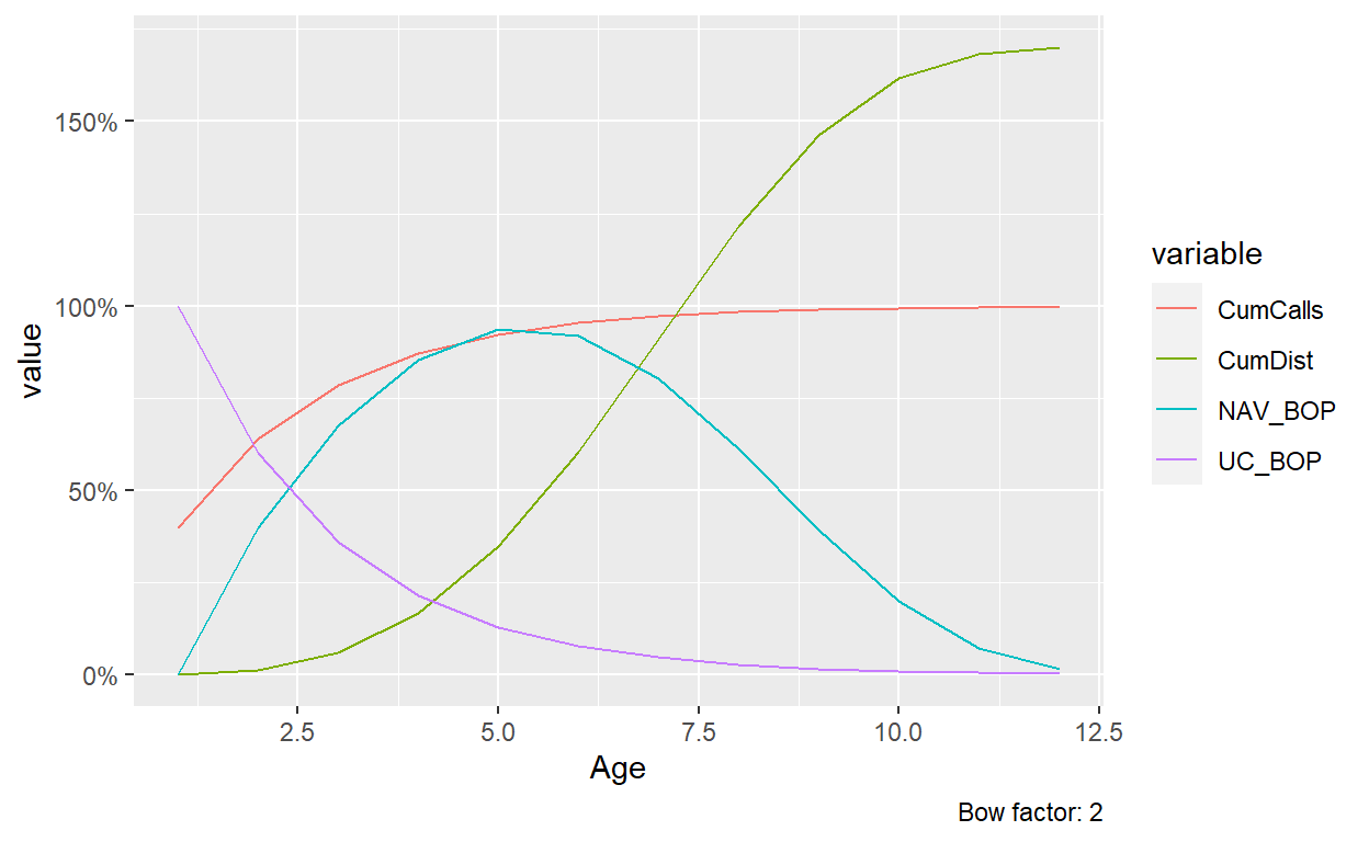
Figure 2: Cumulative calls, distributions, NAV, and unfunded commitment in the TA model. Inputs: bow factor=2, L=12, RC=0.4,G=0.12.
The TVPI and IRR are obtained by calling output_TA$statsTA$TVPIand output_TA$statsTA$IRR, respectively.
Thanks to Rs capabilities, it’s also pretty easy to compare the results for different inputs. For example, let’s look at how the results change for different bow factors, while leaving all the other inputs the same.
Show code
l_results <- lapply(seq(from=0,to=4,by=0.5),
                    run_TA_model,
                       .life=t,
                       .nav=0,
                       .uc=1,
                       .vec_growth = rep(0.12, times=t),
                       .vec_RC =     rep(0.4, times=t))
DT <- rbindlist(l_results)
meltDT <- melt(DT[, list(Age, Bow, CumCalls,CumDist, NAV_BOP)], id.vars = c("Age", "Bow"))
ggplot(meltDT, aes(x=Age, y=value, color=variable)) +
  geom_line() +
  facet_wrap(vars(Bow), nrow=3) + ylab("")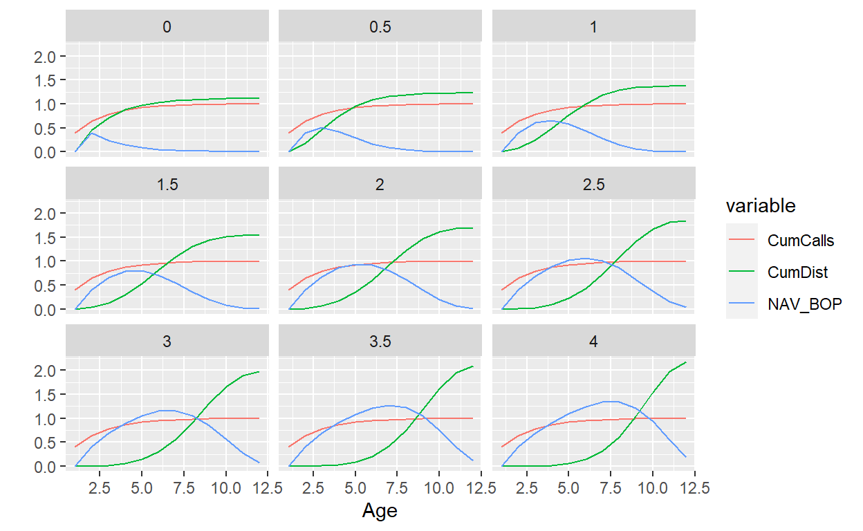
Figure 3: Cumulative calls, distributions, and NAV in the TA model for different bow factors. Inputs: L=12, RC=0.4,G=0.12.
Show code
results_TVPI_IRR <- rbindlist(lapply(l_results, function(x) output_TA_model(x)$statsTA))
results_TVPI_IRR[, Bow:=seq(from=0,to=4,by=0.5)]
library(kableExtra)
kbl(results_TVPI_IRR[,list(Bow,TVPI,IRR)],
    digits=3,
    caption=paste0("TVPI and IRR for different bow factors.")) %>%
kable_classic(full_width = FALSE) | Bow | TVPI | IRR |
|---|---|---|
| 0.0 | 1.118 | 0.119 |
| 0.5 | 1.233 | 0.120 |
| 1.0 | 1.383 | 0.120 |
| 1.5 | 1.547 | 0.120 |
| 2.0 | 1.705 | 0.120 |
| 2.5 | 1.850 | 0.120 |
| 3.0 | 1.978 | 0.120 |
| 3.5 | 2.090 | 0.120 |
| 4.0 | 2.188 | 0.120 |
The higher the bow factor, the more backloaded the distributions are. This implies a higher multiple as there is more time for value creation, while the IRR, or growth rate of value, stays the same, at 12% in this case. The example illustrates nicely that a benchmark based on the TVPI alone is meaningless: a multiple of 2x can either be good or bad, depending on how long it took to generate it.
Final remarks
In this post, I have introduced the TA model and have shown how to implement it in R. Of course, this is the easy part. The much harder part would be the calibration of the model. What parameters should one use to derive reasonable outcomes? To do so, one would have to get real cash flow data of funds and run regressions to estimate the parameters. As the function is non-linear, some adjustments have to be made. My statistic knowledge is diminishing, but this post seems like a good starting point to do so. Fundamentally, the issue I see with calibration is that most funds actually have highly non-linear functions of cash flows, in particular distributions, which do not resemble the curves of the TA model at all. In particular (lower) mid-market buyout funds with only 5-6 investments might not distribute at all in a year or two, just to have large distributions in the next year. Hence, the TA model might therefore be better suited to model portfolio of funds, as the actual curves get the smoother, the more diversified the portfolio is.