Whenever a macroeconomic shock happens, such as the COVID pandemic or Russia’s invasion of Ukraine, investors wonder how companies from certain sectors are impacted. One way is a detailed bottom-up analysis by looking into a particular business in detail and trying to understand how demand, supply chains, labor force, etc. are impacted by the event. However, this is an unrealistic tack for investors with larger portfolios. Fortunately, millions of investors do this exercise as well and trade shares in businesses as a response to their findings. One can piggyback on this work and look at sector indices to get a rough guess on how bad a particular sector and its underlying companies are impacted. In this post, let’s look at two publicly available data sources to do this.
Data from Kenneth French’s website
Kenneth French kindly provides daily updated performance data for different sectors on his website. I wrote a short wrapper function that allows me to download the data from the website and get it into a format I can work with in R. You can find the function in the code chunk below.
Show code
### Load packages that I need later
library(data.table)
library(lubridate)
library(ggplot2)
library(kableExtra)
library(utilitiesCJ)
### Define function
get_FF_data <- function(.str_file, .bol_quarterly=FALSE, ...) {

  ###1. Download data
  temp <- tempfile()
  download.file(.str_file,temp, mode="wb")
  csvDT <- data.table::fread(unzip(temp), ...)
  unlink(temp)


  ###2. Change names of columns
  #     FF doesn't label the date column, enter
  data.table::setnames(csvDT,
           old = "V1",
           new = "Date")
  #     Get rid of hyphens, don't go well with column names
  data.table::setnames(csvDT,
           old = grep("-",names(csvDT),value=TRUE),
           new = gsub("-", "", grep("-",names(csvDT),value=TRUE)))

  ###3. Convert Date column to date; through warning if format changed
  if (sum(is.na(lubridate::ymd(csvDT$Date)))>0) {
    stop("Error in parsing dates to date format: it seems the format in Kenneth French files has changed.")
  }
  csvDT[, Date:=lubridate::ymd(Date)]

  return(csvDT)

}

###Change to the folder you want the data to be downlaoded
setwd("C:/Users/Christoph Jaeckel/Downloads/")
###Go to Kenneth French's website (https://mba.tuck.dartmouth.edu/pages/faculty/ken.french/data_library.html) and get the link to the data file you want to download
### Change link here to play around with other sector classifications
str_file <- "https://mba.tuck.dartmouth.edu/pages/faculty/ken.french/ftp/12_Industry_Portfolios_daily_CSV.zip"
#str_file <- "https://mba.tuck.dartmouth.edu/pages/faculty/ken.french/ftp/17_Industry_Portfolios_daily_CSV.zip"
#str_file <- "https://mba.tuck.dartmouth.edu/pages/faculty/ken.french/ftp/38_Industry_Portfolios_daily_CSV.zip"
#str_file <- "https://mba.tuck.dartmouth.edu/pages/faculty/ken.french/ftp/49_Industry_Portfolios_daily_CSV.zip"
DT <- get_FF_data(str_file, skip = 9, header=TRUE)

### Convert columns to numeric
cols <- names(DT)[2:ncol(DT)]
DT[ , (cols) := lapply(.SD, as.numeric), .SDcols = cols]
# # Calculate the mean daily return (in bps) over the last years
# DT[year(Date)>2010, lapply(.SD, mean), by = year(Date),.SDcols = cols]
#
In this post, I use a classification of 12 sector or industry portfolios. French also has data with lower (only 5 sectors) or higher (12, 17, 30, 38, 48, 49 sectors) granularity on his website. The 12 portfolios are the following:
- NoDur: Consumer Nondurables – Food, Tobacco, Textiles, Apparel, Leather, Toys
- Durbl: Consumer Durables – Cars, TVs, Furniture, Household Appliances
- Manuf: Manufacturing – Machinery, Trucks, Planes, Off Furn, Paper, Com Printing
- Enrgy: Oil, Gas, and Coal Extraction and Products
- Chems: Chemicals and Allied Products
- BusEq: Business Equipment – Computers, Software, and Electronic Equipment
- Telcm: Telephone and Television Transmission
- Utils: Utilities
- Shops: Wholesale, Retail, and Some Services (Laundries, Repair Shops)
- Hlth: Healthcare, Medical Equipment, and Drugs
- Money: Finance
- Other: Other – Mines, Constr, BldMt, Trans, Hotels, Bus Serv, Entertainment
Let’s first look at the average daily returns of those sectors over the last decade in the table below.
Show code
startYear <- 2011
intDT <- DT[year(Date)>=startYear, lapply(.SD, mean), .SDcols = cols]
kbl(intDT,
    digits=3,
    caption=paste0("Average daily returns since ",
                   startYear,
                   " for 12 sectors. Data from Kenneth French's website, obtained on ",
                   today(), ". Numbers in percent.")) %>%
  kable_classic(full_width = FALSE)
| NoDur | Durbl | Manuf | Enrgy | Chems | BusEq | Telcm | Utils | Shops | Hlth | Money | Other |
|---|---|---|---|---|---|---|---|---|---|---|---|
| 0.046 | 0.079 | 0.055 | 0.031 | 0.046 | 0.076 | 0.047 | 0.044 | 0.065 | 0.06 | 0.061 | 0.05 |
These numbers are already shown as percentage. As an example, the BusEq sector returned 0.076% on average per day. Doesn’t sound like a lot, but compounded over 252 days this results in an annualized return of 21.2%.
Let’s now look how the COVID pandemic impacted these sectors.
Initial COVID impact
The S&P 500 declined from close to 3,400 on 21 February 2020 to just over 2,300 on 20 March 2020. How did the different sectors contribute to those massive losses?
Show code
intDT <- melt(DT[Date>=dmy("21022020") & Date<=dmy("20032020")], id.var="Date")[,list(Ret=prod(1+value/100)-1),by=variable]
plotBar(.intDT = intDT,
        .x_name = "variable",
        .y_name = "Ret",
        .x_lab = "Sector",
        .y_lab = "Return",
        .fillColor = "#581845",
        .bolSort = TRUE) +
  scale_y_continuous(labels = scales::percent_format(accuracy = 1)) +
  theme(axis.text.x = element_text(angle = 45, hjust=1))
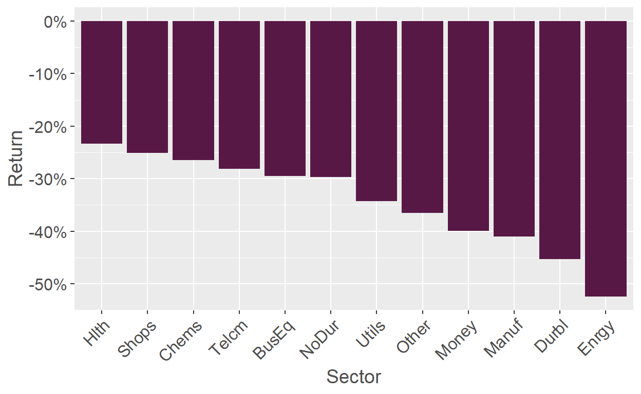
Figure 1: Sector returns from 21 February 2020 to 20 March 2020. Data from Kenneth French’s website.
Healthcare was the most resilient sector in the first phase of the pandemic and only lost slightly over 20%. Shops is an interesting one as many retailers had to close.1 Later on, I show with different data that this sector most likely also includes retailers for daily goods that profited from the panic buying, which explains the overall low impact of the pandemic on this sector. This is a good example of how classifications can lead to ambiguous interpretations.
The most impacted sectors were Durables and Energy. Both these sectors are cyclical sectors and initially there was fear among investors that the pandemic would lead to a recession, so it is not surprising that they were impacted heavily. In case of Energy, it would be interesting if part of the underperformance was also attributed to the expectation of substantially lower travel activities due to the lock down and, as a result, lower fuel consumption.
COVID recovery
The S&P 500 then rose close to 3,800 until the end of the year. Which sectors drove this exceptional recovery? The chart below gives the answer.
Show code
intDT <- melt(DT[Date>dmy("20032020") & Date<=dmy("31122020")], id.var="Date")[,list(Ret=prod(1+value/100)-1),by=variable]
plotBar(.intDT = intDT,
        .x_name = "variable",
        .y_name = "Ret",
        .x_lab = "Sector",
        .y_lab = "Return",
        .fillColor = "#581845",
        .bolSort = TRUE) +
  scale_y_continuous(labels = scales::percent_format(accuracy = 1)) +
  theme(axis.text.x = element_text(angle = 45, hjust=1))
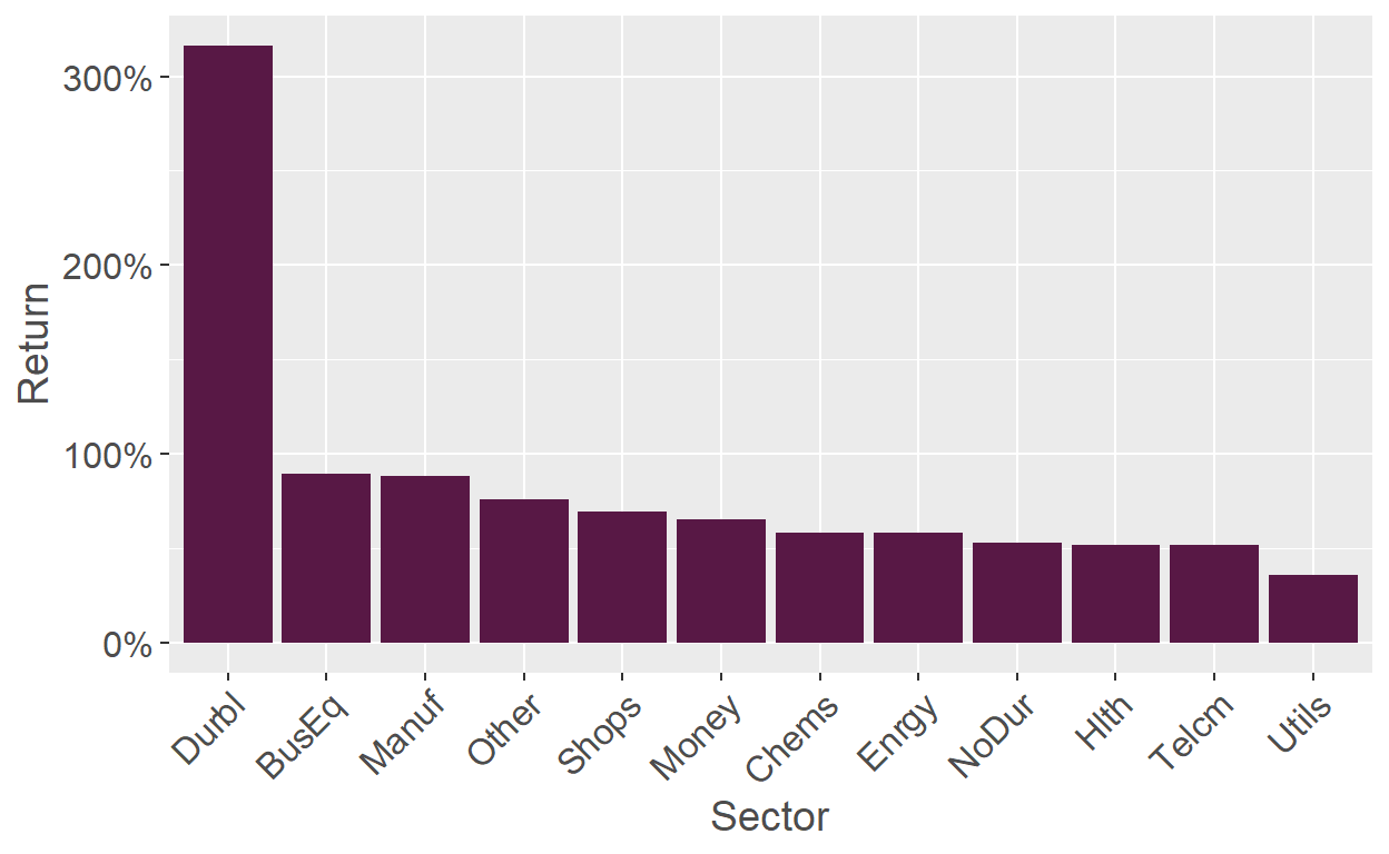
Figure 2: Sector returns from 21 March 2020 to 31 December 2020. Data from Kenneth French’s website.
Durables was by far the best performing sector. It is such an outlier that it would indeed by intersting to know the constituents as my first guess would not have been that companies dealing with “Cars, TVs, Furniture, Household Appliances” were the clear COVID winners. Obviously, Cars include Tesla and Tesla rose over 700% in that period, being one very important driver of this sector, given how large this company’s market cap was at the end of 2020.
Unfortunately, the classifications by French do not really put tech / software companies in one bucket. Obviously, these firms performed exceptionally throughout the pandemic, but I don’t quite know where they ended up. Could be Durables, could be Business Equipment, or something else. Fortunately, the data set I use next shows the sector performance in more granularity.
Data from Aswath Damodaran’s website
In my very first post, I already introduced a function that downloads the data from Damodaran’s website. I use this function here to download his Excel file that documents the COVID impact on U.S. firms.
Show code
setnames(intDT,
         old = c("Industry Name", "Number of firms", "12/31/19", "2/14/20", "3/20/20", "9/1/20", "12/31/21",
                 "1/1/20 -  2/14", "2/14/20 - 3/20/20", "3/20/20 - 9/1/20", "9/1/20 - 12/31/21", "1/1/20 - 12/31/21",
                 "LTM 2020", "LTM 2021", "% Change", "LTM 20202", "LTM 20213", "% Change4"),
         new = c("Sector", "N", "MktCap_31Dec19", "MktCap_14Feb20", "MktCap_20Mar20", "MktCap_1Sep20", "MktCap_31Dec21",
                 "Chg_preCOVID", "Chg_initial", "Chg_Recov", "Chg_end20", "Chg_21",
                 "Rev_LTM_2020", "Rev_LTM_2021", "Chg_Rev", "OpInc_LTM_2020", "OpInc_LTM_2021", "Chg_OpInc"))
## Report
intDT <- intDT[grep("Total Market", Sector,invert =TRUE)]
intDT[, Comb:=(1+Chg_initial)*(1+Chg_Recov)*(1+Chg_end20)-1]
intDT2 <- intDT[,list(Sector, N, Chg_initial, Chg_Recov, Chg_end20, Comb)][order(Chg_initial)]
intDT2[, Rank:=round(rank(-Comb),digits=0)]
cols <- c("Chg_initial", "Chg_Recov", "Chg_end20", "Comb")
intDT2[, (cols) := lapply(.SD, function(x) {paste0(format(round(x*100,digits=1),nsmall=1), "%")}), .SDcols = cols]
kbl(intDT2,
    align = "c",
    col.names = c("Sector", "Nr. of firms", "2/14/20 - 3/20/20", "3/20/20 - 9/1/20", "9/1/20 - 12/31/21", "Combined", "Rank"),
    caption="Performance of different sectors during different phases of the COVID pandemic, sorted by performance in the initial phase. Rank is based on the combined performance. Data from Damodaran's website.") %>%
  kable_classic(full_width = FALSE)
| Sector | Nr. of firms | 2/14/20 - 3/20/20 | 3/20/20 - 9/1/20 | 9/1/20 - 12/31/21 | Combined | Rank |
|---|---|---|---|---|---|---|
| Air Transport | 21 | -60.9% | 49.8% | 46.3% | -14.4% | 92 |
| Real Estate (Development) | 19 | -60.5% | 72.3% | 59.5% | 8.5% | 78 |
| Oilfield Svcs/Equip. | 100 | -58.0% | 50.6% | 58.4% | 0.4% | 88 |
| Oil/Gas (Production and Exploration) | 183 | -57.0% | 56.0% | 161.2% | 75.4% | 27 |
| Food Wholesalers | 15 | -56.9% | 74.3% | 40.5% | 5.6% | 83 |
| Insurance (Life) | 24 | -53.8% | 56.3% | 50.6% | 8.7% | 76 |
| Homebuilding | 29 | -53.8% | 132.5% | 45.8% | 56.6% | 36 |
| Hotel/Gaming | 66 | -53.8% | 72.4% | 79.3% | 42.9% | 51 |
| Oil/Gas Distribution | 21 | -52.9% | 47.2% | 56.3% | 8.4% | 79 |
| Furn/Home Furnishings | 32 | -51.4% | 102.6% | 54.0% | 51.5% | 39 |
| Reinsurance | 2 | -51.2% | 35.4% | 16.3% | -23.2% | 94 |
| Broadcasting | 28 | -49.6% | 40.9% | 25.7% | -10.7% | 90 |
| Rubber& Tires | 2 | -48.7% | 70.3% | 166.1% | 132.3% | 7 |
| Oil/Gas (Integrated) | 4 | -48.4% | 28.6% | 53.7% | 2.1% | 87 |
| Real Estate (Operations & Services) | 51 | -48.1% | 97.8% | 95.6% | 100.7% | 13 |
| Aerospace/Defense | 73 | -48.1% | 37.6% | 22.9% | -12.2% | 91 |
| Hospitals/Healthcare Facilities | 31 | -48.0% | 66.2% | 69.2% | 46.3% | 45 |
| Paper/Forest Products | 11 | -48.0% | 73.8% | 67.3% | 51.3% | 40 |
| Recreation | 60 | -47.6% | 122.6% | 43.3% | 67.0% | 33 |
| Auto & Truck | 26 | -47.3% | 314.3% | 168.4% | 485.6% | 1 |
| Engineering/Construction | 48 | -45.9% | 82.6% | 92.6% | 90.1% | 18 |
| Chemical (Basic) | 35 | -45.7% | 66.8% | 48.3% | 34.4% | 57 |
| Advertising | 49 | -45.1% | 35.1% | 109.4% | 55.2% | 38 |
| Chemical (Diversified) | 4 | -44.4% | 92.7% | 63.9% | 75.6% | 26 |
| Apparel | 39 | -44.1% | 28.0% | 52.0% | 8.6% | 77 |
| Bank (Money Center) | 7 | -44.0% | 18.4% | 55.5% | 3.1% | 85 |
| Metals & Mining | 74 | -43.4% | 122.6% | 94.6% | 145.3% | 6 |
| Office Equipment & Services | 18 | -43.2% | 35.3% | 38.3% | 6.4% | 81 |
| Auto Parts | 38 | -42.2% | 73.7% | 81.4% | 82.2% | 22 |
| Brokerage & Investment Banking | 31 | -42.1% | 49.0% | 127.2% | 96.0% | 16 |
| Banks (Regional) | 563 | -42.1% | 23.6% | 84.8% | 32.2% | 61 |
| Semiconductor Equip | 34 | -41.5% | 79.4% | 113.5% | 123.9% | 8 |
| Insurance (General) | 23 | -41.5% | 45.5% | 62.0% | 37.8% | 56 |
| Shipbuilding & Marine | 8 | -41.5% | 22.8% | 82.9% | 31.5% | 62 |
| Retail (Building Supply) | 16 | -41.1% | 104.2% | 41.7% | 70.6% | 30 |
| Education | 35 | -41.1% | 77.1% | 12.7% | 17.6% | 70 |
| Coal & Related Energy | 18 | -40.8% | 23.7% | 266.6% | 168.6% | 5 |
| Steel | 28 | -40.4% | 56.2% | 116.2% | 101.3% | 12 |
| Retail (Distributors) | 68 | -40.2% | 84.9% | 62.8% | 80.1% | 23 |
| Financial Svcs. (Non-bank & Insurance) | 223 | -40.0% | 49.2% | 57.5% | 41.1% | 53 |
| Retail (Special Lines) | 76 | -39.7% | 47.2% | 55.9% | 38.3% | 55 |
| Investments & Asset Management | 687 | -39.7% | 52.4% | 126.0% | 107.6% | 10 |
| R.E.I.T. | 238 | -39.5% | 36.8% | 53.0% | 26.6% | 69 |
| Retail (Automotive) | 32 | -38.9% | 118.7% | 28.1% | 71.2% | 29 |
| Trucking | 34 | -38.9% | 66.1% | 64.4% | 66.9% | 34 |
| Electrical Equipment | 104 | -38.7% | 79.9% | 71.9% | 89.5% | 19 |
| Electronics (Consumer & Office) | 16 | -38.4% | 76.0% | 286.0% | 318.8% | 3 |
| Restaurant/Dining | 70 | -38.0% | 60.4% | 34.0% | 33.2% | 58 |
| Computer Services | 83 | -38.0% | 42.6% | 44.9% | 28.2% | 68 |
| Real Estate (General/Diversified) | 10 | -37.5% | 30.6% | 90.6% | 55.6% | 37 |
| Transportation (Railroads) | 4 | -37.4% | 63.1% | 28.4% | 31.0% | 64 |
| Shoe | 12 | -36.6% | 70.9% | 51.0% | 63.8% | 35 |
| Machinery | 111 | -36.5% | 68.7% | 40.6% | 50.4% | 41 |
| Business & Consumer Services | 160 | -36.0% | 59.0% | 41.2% | 43.8% | 48 |
| Beverage (Alcoholic) | 21 | -35.3% | 52.2% | 16.3% | 14.6% | 72 |
| Construction Supplies | 48 | -35.2% | 67.0% | 32.1% | 42.9% | 50 |
| Information Services | 79 | -35.1% | 63.8% | 6.4% | 13.1% | 74 |
| Chemical (Specialty) | 81 | -34.2% | 56.3% | 41.4% | 45.4% | 46 |
| Publishing & Newspapers | 21 | -34.1% | 41.2% | 37.8% | 28.2% | 67 |
| Farming/Agriculture | 36 | -34.1% | 69.5% | 58.8% | 77.3% | 25 |
| Insurance (Prop/Cas.) | 52 | -33.8% | 30.8% | 21.8% | 5.4% | 84 |
| Power | 50 | -33.5% | 25.6% | 28.9% | 7.6% | 80 |
| Electronics (General) | 137 | -33.1% | 55.2% | 68.2% | 74.8% | 28 |
| Semiconductor | 67 | -32.0% | 77.2% | 71.7% | 106.9% | 11 |
| Beverage (Soft) | 32 | -31.4% | 33.6% | 23.9% | 13.6% | 73 |
| Utility (General) | 16 | -31.2% | 22.4% | 16.5% | -1.9% | 89 |
| Healthcare Support Services | 131 | -30.8% | 43.1% | 50.4% | 48.9% | 44 |
| Healthcare Products | 244 | -30.7% | 58.0% | 31.0% | 43.5% | 49 |
| Computers/Peripherals | 46 | -30.6% | 122.9% | 28.2% | 98.3% | 15 |
| Software (Entertainment) | 88 | -30.4% | 75.0% | 46.3% | 78.3% | 24 |
| Packaging & Container | 26 | -30.3% | 40.3% | 35.3% | 32.4% | 59 |
| Diversified | 22 | -29.8% | 27.7% | 28.2% | 15.0% | 71 |
| Cable TV | 11 | -29.5% | 40.9% | 3.0% | 2.3% | 86 |
| Building Materials | 44 | -29.5% | 97.5% | 56.4% | 117.9% | 9 |
| Entertainment | 108 | -28.2% | 67.0% | 24.7% | 49.4% | 43 |
| Tobacco | 16 | -28.2% | 27.6% | 16.0% | 6.2% | 82 |
| Software (System & Application) | 375 | -26.7% | 76.1% | 43.3% | 84.9% | 20 |
| Environmental & Waste Services | 58 | -26.5% | 30.6% | 37.7% | 32.2% | 60 |
| Green & Renewable Energy | 20 | -26.2% | 302.3% | 61.2% | 378.7% | 2 |
| Telecom. Equipment | 82 | -25.3% | 24.0% | 61.9% | 49.9% | 42 |
| Utility (Water) | 14 | -23.9% | 24.5% | 35.6% | 28.4% | 66 |
| Heathcare Information and Technology | 142 | -23.5% | 65.3% | 58.2% | 100.1% | 14 |
| Software (Internet) | 36 | -23.5% | 112.1% | 92.1% | 211.9% | 4 |
| Telecom (Wireless) | 17 | -22.7% | 117.5% | -0.1% | 68.0% | 31 |
| Drugs (Pharmaceutical) | 298 | -21.4% | 29.1% | 29.5% | 31.4% | 63 |
| Food Processing | 92 | -21.0% | 30.5% | 8.5% | 11.9% | 75 |
| Household Products | 118 | -20.8% | 35.9% | 21.7% | 31.0% | 65 |
| Telecom. Services | 42 | -20.1% | 9.6% | -9.5% | -20.8% | 93 |
| Transportation | 17 | -17.9% | 78.3% | 33.5% | 95.5% | 17 |
| Drugs (Biotechnology) | 581 | -17.7% | 42.0% | 24.1% | 45.0% | 47 |
| Precious Metals | 76 | -14.7% | 77.6% | -7.9% | 39.5% | 54 |
| Retail (Online) | 60 | -14.6% | 94.6% | 0.6% | 67.1% | 32 |
| Retail (General) | 16 | -9.0% | 31.1% | 19.5% | 42.6% | 52 |
| Retail (Grocery and Food) | 15 | 4.3% | 34.8% | 31.2% | 84.4% | 21 |
Damodaran’s sector classification is much more granular, which confirms some of the hypotheses I made above when looking at French’s data. For example, Shops did reasonably well as some of the clear initial COVID winners were grocery and food retailers. Shoes and apparel shops, on the other hand, suffered substantially.
The table also shows nicely for which sectors the sentiment stayed relatively constant and for which it changed. Air Transport is a sector that was initially hit the worst and has not recovered grounds since then in comparison to other sectors. Other sectors, such as Oil/Gas (Production and Exploration), did terrible at the start, but ended 2020 as one of the stronger sectors.
Again, Tesla shows up as the clear anomaly in this data set, pushing Auto & Truck to the best performing sector. For me, this is difficult to explain: in an unexpected pandemic, one would have expected certain sector rotations. Air Transport becomes less relevant as people don’t travel anymore; Software and Entertainment profits as people stay at home. Why do cars though become out of a sudden so much more relevant during a pandemic? People always had them, it’s hard for me to come up with a story as to why they became so much more relevant during COVID. Of course, one could argue that the rise of Tesla co-incided with the pandemic, but in this case one would expect the other car manufacturers to lose just as much. Essentially an intra-sector rotation away from the old manufacturers towards Tesla. This, however, didn’t seem to happen either as Tesla gained so much to move the whole sector towards new heights. One explanation could be that Tesla took those gains from non-U.S. competitors such as Daimler, BMW, or Toyota. However, Toyota’s share price increased and most of the others are flat compared to the pandemic.
Damodaran also shows the change in revenues and operating income from 2020 to 2021 and the scatterplots below compare them to the stock market performance from mid-February 2020 to the end of 2020. A strong correlation would indicate that the stock price movements were anticipating subsequent moves in cash flows. However, there is no such correlation visible in the data.
Show code
ggplot(intDT[!is.na(Chg_Rev)],
       aes(x=Comb, y=Chg_Rev)) + #, color=sector_group)) +
  scale_x_continuous(labels = scales::percent)  +
  scale_y_continuous(labels = scales::percent_format(accuracy = 1))  +
  geom_point() + xlab("Stock return: 2/14/20-12/31/20") + ylab("Change Rev 20-21") +
  geom_smooth(method=lm, se=FALSE) +
  theme(legend.title = element_blank())
ggplot(intDT[!is.na(Chg_OpInc)],
       aes(x=Comb, y=Chg_OpInc)) + #, color=sector_group)) +
  scale_x_continuous(labels = scales::percent)  +
  scale_y_continuous(labels = scales::percent_format(accuracy = 1))  +
  geom_point() + xlab("Stock return: 2/14/20-12/31/20") + ylab("Change OpInc 20-21") +
  geom_smooth(method=lm, se=FALSE) +
  theme(legend.title = element_blank())
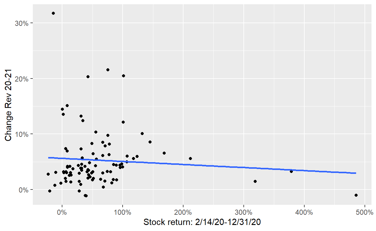
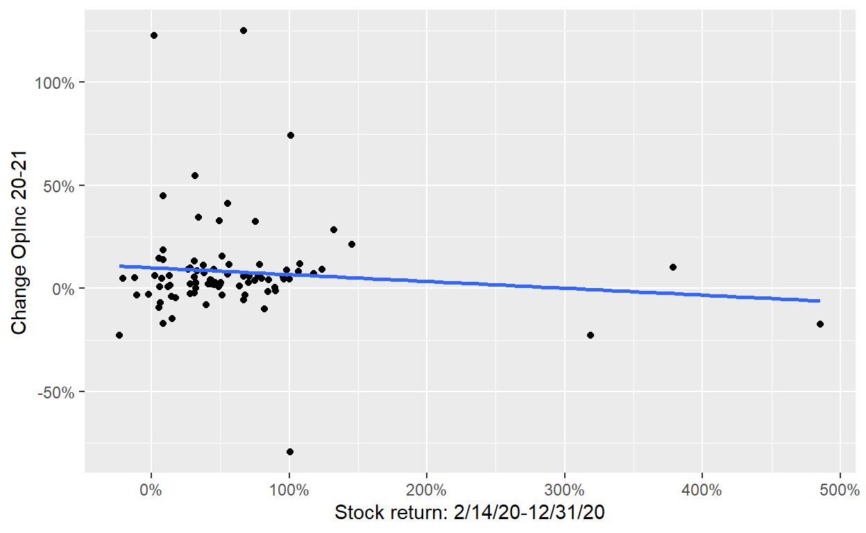
Figure 3: Sector performance from 14 Feb 2020 to 31 Dec 2020 vs. change in revenues and operating income from 2020 to 2021. Data obtained from Damodaran’s website.
Summary
This post has shown how to leverage publicly available data to understand the impact of a macroeconomic shock on different sectors. It used the COVID pandemic as an example, but the code is easily adjustable to look at other events as well.
This Wikipedia article mentions that Apple and many other players closed all their shops on March 14. Hence, investors were already well aware of the dramatic impact of the pandemic on retail.↩︎